0 参考资料
- Pandas中文文档
- NumPy中文文档
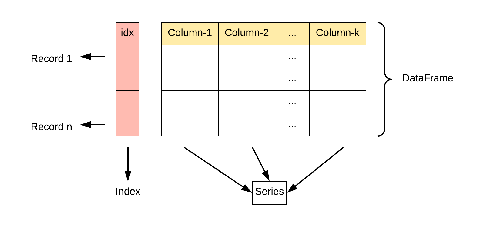
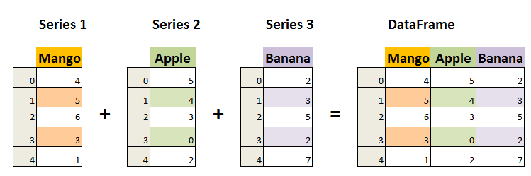
1 Pandas 数据处理
1.1 Pandas 数据结构 - Series
Pandas Series 类似表格中的一个列(column),类似于一维数组,可以保存任何数据类型。
Series 由索引(index)和列组成,函数如下:
1
| pandas.Series( data, index, dtype, name, copy)
|
参数说明:
- data:一组数据(ndarray 类型)。
- index:数据索引标签,如果不指定,默认从 0 开始。
- dtype:数据类型,默认会自己判断。
- name:设置名称。
- copy:拷贝数据,默认为 False。
示例:
1
2
3
4
5
6
7
8
9
10
11
12
13
14
15
16
17
18
19
20
21
22
23
24
25
26
27
28
29
|
pd.Series(['a', 'b', 'c'])
s1 = pd.Series({'a':11, 'b':22, 'c':33})
s2 = pd.Series([11, 22, 33], index = ['a', 'b', 'c'])
print(s1)
print(s2['a'])
print(s2.index)
print(s2.values)
print(type(s1.values))
print(type(np.array(['a', 'b'])))
s2.values.tolist()
|
使用map函数,处理Series中的值,生成新的Series:
1
2
3
4
5
6
7
8
9
10
11
12
13
14
|
emails = pd.Series(['abc at amazom.com', 'admin1@163.com', 'mat@m.at', 'ab@abc.com'])
import re
pattern ='[A-Za-z0-9._]+@[A-Za-z0-9.-]+\\.[A-Za-z]{2,5}'
mask = emails.map(lambda x: bool(re.match(pattern, x)))
print(mask)
print(emails[mask])
|
Pandas通过index可以提升查询性能:
- 如果index唯一,pandas会使用哈希表优化,查询性能为O(1)
- 如果index有序不唯一,pandas会使用二分查找算法,查询性能为O(logN)
- 如果index完全随机,每次查询都要扫全表,查询性能为O(N)
1.2 Pandas 数据结构 - DataFrame
DataFrame 是一个表格型的数据结构,它含有一组有序的列,每列可以是不同的值类型(数值、字符串、布尔型值)。DataFrame 既有行索引也有列索引,它可以被看做由 Series 组成的字典(共同用一个索引)。
1
| pandas.DataFrame( data, index, columns, dtype, copy)
|
参数说明:
- data:一组数据(ndarray、series, map, lists, dict 等类型)。
- index:索引值,或者可以称为行索引。
- columns:列索引,默认为 RangeIndex (0, 1, 2, …, n) 。
- dtype:数据类型。
- copy:拷贝数据,默认为 False。
示例:
1
2
3
4
5
6
7
8
9
10
11
12
13
14
15
16
17
18
19
20
21
22
23
24
25
26
27
28
| import pandas as pd
df1 = pd.DataFrame(['a', 'b', 'c', 'd'])
df2 = pd.DataFrame([
['a', 'b'],
['c', 'd']
])
df2.columns= ['one', 'two']
df2.index = ['first', 'second']
print(df2)
print(df2.columns)
print(df2.index)
print(type(df2.values))
print(df2.values.tolist())
|
1.3 数据导入
Pandas支持大量格式的导入,使用的是read_*() 的形式,如:
1
2
3
4
5
6
7
8
9
10
11
12
13
14
15
16
17
18
19
20
21
22
23
24
25
26
27
28
29
30
31
32
33
34
| import pandas as pd
excel1 = pd.read_excel(r'1.xlsx')
print(excel1)
print(excel1.head(2))
print(excel1.shape)
print(excel1.describe())
pd.read_excel(r'1.xlsx',sheet_name = 0)
pd.read_csv(r'book_utf8.csv',sep=',', nrows=10, encoding='utf-8')
pd.read_table( r'file.txt' , sep = ' ')
import pymysql
sql = 'SELECT * FROM mytable'
conn = pymysql.connect('ip','name','pass','dbname','charset=utf8')
df = pd.read_sql(sql,conn)
|
pd.read_excel(r'1.xlsx',sheet_name = 0) 导入excel,并且指定sheetpd.read_sql(sql,conn) 导入数据库
1.4 数据预处理
处理缺失值
isnull(): 返回布尔值DataFrame,指示每个元素是否为缺失值。示例: df.isnull()fillna(value): 用指定值填充缺失值。示例: df.fillna(0)dropna(): 删除包含缺失值的行或列。示例: df.dropna()
处理重复值
duplicated(): 返回布尔Series,指示是否为重复行。示例: df.duplicated()drop_duplicates(): 删除DataFrame中的重复行。示例: df.drop_duplicates()
处理异常值
- 标识或替换超出范围的值为缺失值:
df[(df < low) | (df > high)] = np.nandf.replace(value_to_replace, new_value)
示例:
1
2
3
4
5
6
7
8
9
10
11
12
13
14
15
16
17
18
19
20
21
22
23
24
25
26
27
28
29
30
31
32
33
34
35
36
37
38
39
40
41
42
43
44
45
46
47
48
49
50
| import pandas as pd
import numpy as np
x = pd.Series([ 1, 2, np.nan, 3, 4, 5, 6, None, 8])
print(x.hasnans)
print(x.isnull())
x.fillna(value = x.mean())
df3=pd.DataFrame({"A":[5,3,None,4],
"B":[None,2,4,3],
"C":[4,3,8,5],
"D":[5,4,2,None]})
df3.isnull().sum()
df3.ffill()
df3.ffill(axis=1)
df3.info()
df3.dropna()
df3.fillna('无')
df3.drop_duplicates()
|
DataFrame的数据调整:
1
2
3
4
5
6
7
8
9
10
11
12
13
14
15
16
17
18
19
20
21
22
23
24
25
| import pandas as pd
df = pd.DataFrame({"A":[5,3,None,4],
"B":[None,2,4,3],
"C":[4,3,8,5],
"D":[5,4,2,None]})
print(df[ ['A', 'C'] ])
print(df.iloc[:, [0,2]])
print(df.loc[ [0, 2] ])
print(df.loc[ 0:2 ])
print(df[ ( df['A']<5 ) & ( df['C']<4 ) ])
print(df.T)
|
1.6 计算操作
1.6.1 基本操作
1
2
3
4
5
6
7
8
9
10
11
12
13
14
15
16
17
18
19
20
21
22
23
24
25
26
27
28
| import pandas as pd
df = pd.DataFrame({"A":[5,3,None,4],
"B":[None,2,4,3],
"C":[4,3,8,5],
"D":[5,4,2,None]})
print(df['A'] + df['C'])
print(df['A'] + 5)
print(df['A'] > df ['C'])
print(df.count())
df.sum()
df['A'].sum()
|
1.6.2 聚合计算
1
2
3
4
5
6
7
8
9
10
11
12
13
14
15
16
17
18
19
20
21
22
23
24
25
26
27
28
29
30
31
32
33
34
35
36
37
38
39
40
41
42
43
44
45
46
47
48
49
50
51
52
| import pandas as pd
import numpy as np
sales = [{'account': 'Jones LLC','type':'a', 'Jan': 150, 'Feb': 200, 'Mar': 140},
{'account': 'Alpha Co','type':'b', 'Jan': 200, 'Feb': 210, 'Mar': 215},
{'account': 'Blue Inc','type':'a', 'Jan': 50, 'Feb': 90, 'Mar': 95 }]
df2 = pd.DataFrame(sales)
print(df2.groupby('type').groups)
for a, b in df2.groupby('type'):
print(a)
print(b)
df2.groupby('type').count()
df2.groupby('type').aggregate( {'type':'count' , 'Feb':'sum' })
group=['x','y','z']
data=pd.DataFrame({
"group":[group[x] for x in np.random.randint(0,len(group),10)] ,
"salary":np.random.randint(5,50,10),
"age":np.random.randint(15,50,10)
})
data.groupby('group').agg('mean')
data.groupby('group').mean().to_dict()
data.groupby('group').transform('mean')
pd.pivot_table(data,
values='salary',
columns='group',
index='age',
aggfunc='count',
margins=True
).reset_index()
|
1.6.3 多表组合
1
2
3
4
5
6
7
8
9
10
11
12
13
14
15
16
17
18
19
20
21
22
23
24
25
26
27
28
29
30
31
32
33
34
35
36
37
38
| import pandas as pd
import numpy as np
group = ['x','y','z']
data1 = pd.DataFrame({
"group":[group[x] for x in np.random.randint(0,len(group),10)] ,
"age":np.random.randint(15,50,10)
})
data2 = pd.DataFrame({
"group":[group[x] for x in np.random.randint(0,len(group),10)] ,
"salary":np.random.randint(5,50,10),
})
data3 = pd.DataFrame({
"group":[group[x] for x in np.random.randint(0,len(group),10)] ,
"age":np.random.randint(15,50,10),
"salary":np.random.randint(5,50,10),
})
pd.merge(data1, data2)
pd.merge(data3, data2, on='group')
pd.merge(data3, data2)
pd.merge(data3, data2, left_on= 'age', right_on='salary')
pd.merge(data3, data2, on= 'group', how='inner')
pd.concat([data1, data2])
|
1.6.4 输出和绘图
1
2
3
4
5
6
7
8
9
10
11
12
13
14
15
16
17
18
19
20
21
22
23
24
25
26
27
28
29
30
|
df.to_excel( excel_writer = r'file.xlsx')
df.to_excel( excel_writer = r'file.xlsx', sheet_name = 'sheet1')
df.to_excel( excel_writer = r'file.xlsx', sheet_name = 'sheet1', index = False)
df.to_excel( excel_writer = r'file.xlsx', sheet_name = 'sheet1',
index = False, columns = ['col1','col2'])
enconding = 'utf-8'
na_rep = 0
inf_rep = 0
to_csv()
df.to_pickle('xx.pkl')
agg(sum)
agg(lambda x: x.sum())
|
1
2
3
4
5
6
7
8
9
10
11
12
13
14
15
16
17
18
19
20
21
22
23
24
25
26
27
28
29
30
31
32
33
34
35
36
37
38
39
40
41
42
43
| import pandas as pd
import numpy as np
dates = pd.date_range('20200101', periods=12)
df = pd.DataFrame(np.random.randn(12,4), index=dates, columns=list('ABCD'))
df
import matplotlib.pyplot as plt
plt.plot(df.index, df['A'], )
plt.show()
plt.plot(df.index, df['A'],
color='#FFAA00',
linestyle='--',
linewidth=3,
marker='D')
plt.show()
import seaborn as sns
plt.scatter(df.index, df['A'])
plt.show()
sns.set_style('darkgrid')
plt.scatter(df.index, df['A'])
plt.show()
|
2 Numpy 使用
2.1 Ndarray对象
NumPy 最重要的一个特点是其 N 维数组对象 ndarray,它是一系列同类型数据的集合,以 0 下标为开始进行集合中元素的索引。ndarray 对象是用于存放同类型元素的多维数组。ndarray 中的每个元素在内存中都有相同存储大小的区域。ndarray 内部由以下内容组成:
- 一个指向数据(内存或内存映射文件中的一块数据)的指针。
- 数据类型或 dtype,描述在数组中的固定大小值的格子。
- 一个表示数组形状(shape)的元组,表示各维度大小的元组。
- 一个跨度元组(stride),其中的整数指的是为了前进到当前维度下一个元素需要”跨过”的字节数。
ndarray 的内部结构:

np.array() 函数:使用 Python 列表或元组创建数组。np.zeros() 和 np.ones() 函数:创建特定形状的全零数组或全一数组。
1
2
3
4
|
zeros_arr = np.zeros((3, 4))
ones_arr = np.ones((3, 4))
|
np.empty() 函数:创建指定形状的未初始化数组。
1
2
|
empty_arr = np.empty((2, 2))
|
np.arange() 函数:类似于 Python 的 range() 函数,创建一个指定范围内的数组。
1
2
|
arr_range = np.arange(0, 10, 2)
|
np.linspace() 函数:创建指定范围内均匀间隔的数组。
1
2
|
arr_linspace = np.linspace(0, 10, 5)
|
np.random 模块:生成随机数组。
1
2
|
rand_int_arr = np.random.randint(1, 100, size=(3, 3))
|
1
2
|
rand_float_arr = np.random.rand(2, 2)
|
1
2
3
4
5
|
rand_normal_arr = np.random.randn(2, 2)
|
2.2 Ndarray 的操作方法
1
2
3
4
5
6
7
8
9
10
11
12
13
14
15
16
17
18
19
| X = np.arange(15).reshape(3,5)
x = np.arange(10)
x.ndim
X.ndim
x.shape
X.shape
x.size
X.size
|
1
2
3
4
5
6
7
8
9
10
11
12
13
14
15
16
17
18
19
20
21
22
23
24
25
26
27
28
29
30
31
32
33
34
35
36
37
38
39
40
41
42
43
44
45
46
|
x[::2]
X[ (1,1) ]
X[1,1]
X[:2, :3]
subarray = X[:2, :3]
subarray[1][1] = 100
subX = X[:2, :3].copy()
a = np.arange(10)
a.reshape(2,5)
a.reshape(10,-1)
x = np.array([1,2,3])
y = np.array([4,5,6])
np.concatenate([x, y])
np.vstack([x, y])
np.hstack([x, y])
x = np.arange(10)
x1, x2, x3 = np.split(x, [3,7])
A = np.arange(16).reshape([4,4])
A1, A2 = np.split(A, [2])
A1, A2 = np.split(A, [2], axis=1)
A1, A2 = np.vsplit(A, [2])
A1, A2= np.hsplit(A, [2])
|
2.3 numpy.array 中的聚合运算
- np.percentile(big_array, q=50) :百分位点,相当于求50%位点
- np.var(big_array):方差,是每个样本值与全体样本值的平均数之差的平方值的平均数,即
mean((x - x.mean())** 2)。
- np.std(big_array):标准差,标准差是一组数据平均值分散程度的一种度量。标准差是方差的算术平方根。
- np.median(big_array):中位数
- np.mean():平均数
numpy.average(a, axis=None, weights=None, returned=False) :函数根据在另一个数组中给出的各自的权重计算数组中元素的加权平均值。 - np.bincount:众数
- np.prod:大数
- np.argmax():返回最大值的索引
- np.argmin()
- np.random.shuffle(x):乱序处理
- np.sort(x):排序,x 未修改
- x.sort():原地排序,x 被修改
- np.sort(x, axis=0):每行排序
- np.sort(x, axis=1):每列排序
- np.argsort(x):排序数组,返回的是元素索引
- np.partition(x, 3):快排中的partition逻辑,返回的数组中,3 前边的数据都小于3,3后边的元素都大于3
- np.argpartition(x, 3):与上边的一样,只是返回的索引
2.4 FancyIndexing
1
2
3
4
5
6
7
8
9
10
11
12
13
14
15
16
17
| X = np.arange(16).reshape(4,4)
ind = np.array([[0,2],
[1,3]])
X[ind]
row = np.array([0,1,2])
col = np.array([1,2,3])
X[row, col]
col = [True, False, True, True]
X[1:3, col]
|
1
2
3
4
5
6
7
8
9
10
11
12
13
14
15
16
17
18
19
| x = np.arange(16)
x < 3
2 * x == 24-4 * x
X[X[:,2] > 3, :]
np.sum(X>3)
np.sum(X > 3, axis=0)
np.sum(X > 3, axis=1)
np.any(X < 0)
np.all(X < 0)
np.sum((X>3) & (X < 10))
np.sum(~(X==0))
|
2.5 视图和副本
副本是一个数据的完整的拷贝,如果我们对副本进行修改,它不会影响到原始数据,物理内存不在同一位置。
视图是数据的一个别称或引用,通过该别称或引用亦便可访问、操作原有数据,但原有数据不会产生拷贝。如果我们对视图进行修改,它会影响到原始数据,物理内存在同一位置。
视图一般发生在:
- 1、numpy 的切片操作返回原数据的视图。
- 2、调用 ndarray 的 view() 函数产生一个视图。
副本一般发生在:
- Python 序列的切片操作,调用deepCopy()函数。
- 调用 ndarray 的 copy() 函数产生一个副本。
视图示例:
1
2
3
4
5
6
7
8
9
10
11
12
| a = np.arange(6).reshape(3,2)
b = a.view()
print(a)
b.shape = 2,3
print(b)
b[0][0] = 100
|
副本示例:
1
2
3
4
| x = np.arange(6).reshape(2,3)
y = x.copy()
y[0][0]=100
|
2.6 Numpy线性代数
| 函数 |
描述 |
dot |
两个数组的点积,即元素对应相乘。 |
vdot |
两个向量的点积 |
inner |
两个数组的内积 |
matmul |
两个数组的矩阵积 |
determinant |
数组的行列式 |
solve |
求解线性矩阵方程 |
inv |
计算矩阵的乘法逆矩阵 |
3 Matplotlib 使用
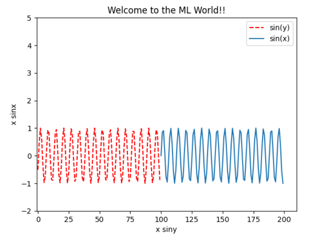
3.1 折线图
1
2
3
4
5
6
7
8
9
10
11
12
13
| import numpy as np
import matplotlib.pyplot as plt
plt.plot(x, siny, color='red', linestyle='--', label='sin(y)')
plt.plot(y, sinx, label='sin(x)')
plt.axis([-1, 210, -2, 5])
plt.legend()
plt.xlabel("x siny")
plt.ylabel("x sinx")
plt.title("Welcome to the ML World!!")
plt.show()
|
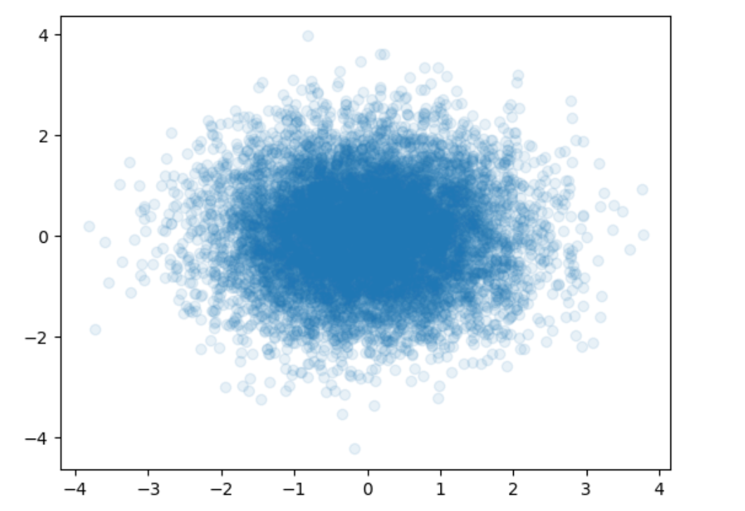
3.2 散点图
1
2
3
4
| x = np.random.normal(0, 1, 10000)
y = np.random.normal(0, 1, 10000)
plt.scatter(x, y, alpha=0.1)
plt.show()
|
4 数据加载和数据处理
1
2
3
4
5
6
7
8
9
10
11
| import numpy as np
import matplotlib as mpl
import matplotlib.pyplot as plt
from sklearn import datasets
iris = datasets.load_iris()
iris.keys()
iris.data
iris.data.shape
iris.target
|
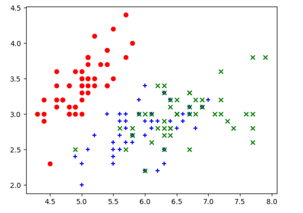
通过数据集绘图:
1
2
3
4
5
6
| X = iris.data
y = iris.target
plt.scatter(X[y==0,0], X[y==0,1], color='red', marker='o')
plt.scatter(X[y==1,0], X[y==1,1], color='blue', marker='+')
plt.scatter(X[y==2,0], X[y==2,1], color='green', marker='x')
plt.show()
|